One can do quite a bit from multivariate summary statistics, but that depends on you giving the intrepid reader all the requisite summary statistics. I have been on this particular soapbox since at least 1991:
Konigsberg LW. 1991. An historical note on the t-test for differences in sexual dimorphism between populations. Am J Phys Anthropol 84:93-96.
So let's turn back the time machine to the late 80s (some pretty awful music back then, I can tell you) and use R to look at sexual dimorphism in LDL and apoB levels in baboons on a regular chow diet as versus a "challenge diet" (called "pink" because loading the monkey chow with cholesterol turned it pink). I can guarantee you that I do not have that raw data anymore, but I did when I wrote the 1991 AJPA "Notes and Comments."
So paste the requisite summary stats into "R":baboons = structure(list(R.res = structure(c(1, 0.487002, 0.681163, 0.476761,
0.487002, 1, 0.326327, 0.804516, 0.681163, 0.326327, 1, 0.399609,
0.476761, 0.804516, 0.399609, 1), .Dim = c(4L, 4L)), M.mu = structure(c(46.4487,
43.2333, 40.9091, 97.4231, 106.1, 87.5454, 39.3833, 37.6755,
35.9909, 57.959, 58.1111, 47.8772), .Dim = 3:4, .Dimnames = list(
c("anubis", "hybrid", "cyno"), c("LDLChow", "LDLpink", "ApoBChow",
"ApoBpink"))), F.mu = structure(c(55.0232, 48.5135, 48.5227,
105.749, 101.9189, 114.7045, 49.0575, 42.9811, 42.1795, 67.7031,
59.3252, 58.4773), .Dim = 3:4, .Dimnames = list(c("anubis", "hybrid",
"cyno"), c("LDLChow", "LDLpink", "ApoBChow", "ApoBpink"))), m = c(78,
90, 22), f = c(259, 111, 44), M.sdev = structure(c(17.1983, 17.4749,
20.8599, 41.4364, 54.5311, 40.6644, 13.9573, 12.9743, 16.0057,
21.8897, 22.4638, 16.8267), .Dim = 3:4), F.sdev = structure(c(17.1913,
20.7596, 23.6992, 44.1428, 51.2467, 65.2397, 14.788, 13.9412,
13.4013, 21.459, 20.8992, 24.0234), .Dim = 3:4)), .Names = c("R.res",
"M.mu", "F.mu", "m", "f", "M.sdev", "F.sdev"))
And list to the screen so we can see what this stuff is and understand the use of the "$" symbol within a list.
baboons
$R.res
[,1] [,2] [,3] [,4]
[1,] 1.000000 0.487002 0.681163 0.476761
[2,] 0.487002 1.000000 0.326327 0.804516
[3,] 0.681163 0.326327 1.000000 0.399609
[4,] 0.476761 0.804516 0.399609 1.000000
$M.mu
LDLChow LDLpink ApoBChow ApoBpink
anubis 46.4487 97.4231 39.3833 57.9590
hybrid 43.2333 106.1000 37.6755 58.1111
cyno 40.9091 87.5454 35.9909 47.8772
$F.mu
LDLChow LDLpink ApoBChow ApoBpink
anubis 55.0232 105.7490 49.0575 67.7031
hybrid 48.5135 101.9189 42.9811 59.3252
cyno 48.5227 114.7045 42.1795 58.4773
$m
[1] 78 90 22
$f
[1] 259 111 44
$M.sdev
[,1] [,2] [,3] [,4]
[1,] 17.1983 41.4364 13.9573 21.8897
[2,] 17.4749 54.5311 12.9743 22.4638
[3,] 20.8599 40.6644 16.0057 16.8267
$F.sdev
[,1] [,2] [,3] [,4]
[1,] 17.1913 44.1428 14.7880 21.4590
[2,] 20.7596 51.2467 13.9412 20.8992
[3,] 23.6992 65.2397 13.4013 24.0234
And a script to do the analysis (that was 1000+ lines of Fortran code back in the day, though thankfully I didn't have to write most of it).
Kberg91 = function (dat=baboons)
{
R = dat$R.res
M = dat$M.mu; F = dat$F.mu
nM = dat$m; nF = dat$f
M.sd = dat$M.sdev; F.sd = dat$F.sdev
p=NROW(R)
r=NROW(M)
o.p=rep(1,p)
o.r=rep(1,r)
J=matrix(1,nr=r,nc=r)
d=M-F
N = sum(nM)+sum(nF)
w=(nM*nF)/(nM+nF)
SSCPsex=t(d)%*%w%*%t(w)%*%d/as.numeric(t(o.r)%*%w)
SSCPi=t(d)%*%(w%*%t(o.p)*d)-SSCPsex
T=diag(sqrt(apply((nM-1)%o%o.p*M.sd^2 + (nF-1)%o%o.p*F.sd^2,2,sum)))
SSCPe=T%*%R%*%T
Xm=nM%*%t(o.p)*M
Xf=nF%*%t(o.p)*F
SSCPsamp = t(Xm)%*%M + t(Xf)%*%F - t(Xm)%*%J%*%Xm/sum(nM) -
t(Xf)%*%J%*%Xf/sum(nF) - SSCPi
Lambda = det(SSCPe)/det(SSCPi+SSCPe)
Lambda[2] = det(SSCPi+SSCPe)/det(SSCPsex+SSCPi+SSCPe)
Lambda[3] = det(SSCPi+SSCPe)/det(SSCPsamp+SSCPi+SSCPe)
vh = r - 1
vh[2] = 1
vh[3] = vh[1]
ve = N - 2*r
ve[2] = N - 2*(r-1)
ve[3] = ve[2]
m = ve + vh - (p + vh + 1)/2
s = sqrt(((p*vh)^2-4)/(p^2+vh^2-5))
df1 = p*vh
df2 = m*s-p*vh/2+1
Rao.R = (1-Lambda^(1/s))/(Lambda^(1/s))*(m*s-p*vh/2+1)/(p*vh)
p = 1-pf(Rao.R,df1,df2)
out = cbind(round(Lambda,4),round(Rao.R,4),round(df1,0),round(df2,0),round(p,4))
rownames(out)=c('Sex*Subspec','Sex','Subsp')
colnames(out)=c("Wilks' Lambda","Rao's R",'df1','df2','Prob')
out
}
Kberg91()
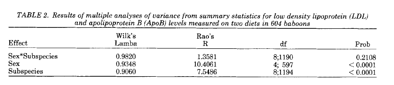
Wilks' Lambda Rao's R df1 df2 Prob
Sex*Subspec 0.9820 1.3581 8 1190 0.2108
Sex 0.9348 10.4061 4 597 0.0000
Subsp 0.9060 7.5486 8 1194 0.0000
Which shows that there is significant sexual dimorphism and differences between the subspecies, but no sex-by-subspecies interaction.
Here's the published results from AJPA in 1991:
The simplest of pdfs, and some calculus
The harsh (?) reality is that most of us are more comfy-cozy with continuous density functions, also known as "probability density functions" or just pdfs (which is confusing what with Adobe Acrobat having subverted the acronym). And among our most favorite pdf is probably (intentional pun) the normal pdf. But that is a two parameter pdf (mean and variance), so let's instead start simple and spend some quality time with the uniform pdf.
...and what is that "and some calculus" bit about? Not to worry. "R" and "SimPy Gamma" will be doing the heavy lifting for us. I generally use wxMaxima for all my calculus and algebraic needs, but SimPy Gamma is a quick on-line way to go.
The uniform (rectangular) pdf
I have sometimes walked into defenses with the bald-faced claim that I have an age-at-death estimation method that never fails, which is to say that the age was between 0 and 120 years. So let's take that as our first uniform distribution.
R has the uniform built in as one of many pdfs. So let's first get some info:
?dunif
| Uniform {stats} | R Documentation |
The Uniform Distribution
Description
These functions provide information about the uniform distribution on the interval from min to max. dunif gives the density, punif gives the distribution function qunif gives the quantile function and runif generates random deviates.
Usage
dunif(x, min = 0, max = 1, log = FALSE).
punif(q, min = 0, max = 1, lower.tail = TRUE, log.p = FALSE)
qunif(p, min = 0, max = 1, lower.tail = TRUE, log.p = FALSE)
runif(n, min = 0, max = 1)
.
.
So what is the median of our ~U(0,120) pdf? Another way of asking this is what is the 50th percentile value? Should be smack dab in the middle, so age 60, but we can use "qunif" to check this (and get the 25th and 75th percentiles as well):
qunif(p=c(.25,.5,.75),0,120)
[1] 30 60 90
So what is the mean of our ~U(0,120) pdf? It is also 60.
mu.unif = function (x)
{
x*dunif(x,0,120)
}
integrate(mu.unif,0,120)
60 with absolute error < 6.7e-13
So we have seen quinf and dunif. Speaking of which, R told us in the help above that dunif was the (probability) density (function). In symbols, this is usually written as f(x). So what is f(10), f(34.34), f(0), f(120), f(121), etc.?
dunif(10,0,120)
[1] 0.008333333
1/120
[1] 0.008333333
And what is runif?
hist(runif(10000,0,120),pr=T,ylim=c(0,0.01))
abline(h=1/120)
And punif? It is the cumulative density function which is also known as the distribution function. It is the "p-value" that you have butted heads (but not tails?) with in stats classes. In symbols, it is usually written as F(x)
punif(0,0,120)
[1] 0
punif(60,0,120)
[1] 0.5
punif(90,0,120)
[1] 0.75
But wait, there's more! You can also use punif to find the complement, which is sometimes referred to as the survivorship function. In symbols, this is usually written as S(x), and it is equal to 1 - F(x)
plot(0:120,punif(0:120,0,120,lower=F),type='l')
But wait, there's more ---- that believe it or not is not in R, and that would be the hazard function. From "hazards analysis" we have f(x) = S(x)h(x), which if you know your abridged life table notation is the continuous analog of d(x) = l(x)q(x) where d(x) is the proportion of deaths in the age interval, l(x) is survivorship to the beginning of the interval, and q(x) is the age-specific probability of death for the interval. So h(x) is sort of like a probability, except that it can be greater than 1.0 (so it is the "hazard rate"). Solving for h(x), we can plot it using dunif divided by 1-punif.
plot(0:120,dunif(0:120,0,120)/(1-punif(0:120,0,120)),type='l')
From hazards analysis, h(x) is also the negative of the first derivative of log survivorship, which turns out to be 1/(120-x). We will try to get this using "SimPy Gamma" copy: diff(log(1-x/120),x) and paste to simpy. That gave you the derivative, so negate to get: 1/(120-x)
In wxMaxima it looks like so:
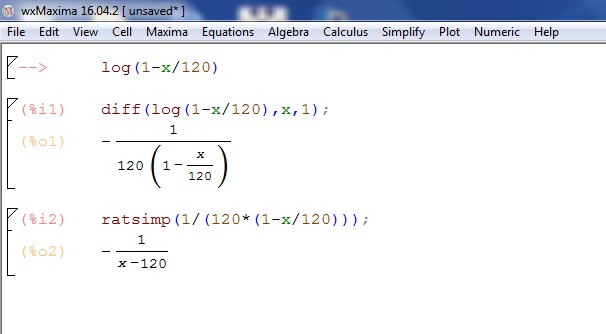
lines(0:120,1/(120-(0:120)),col='red')
Out of curiosity, what is the variance of U(0,120)?
var.unif = function (x)
{
(x-60)^2*(1/120)
}
integrate(var.unif,0,120)
1200 with absolute error < 1.3e-11
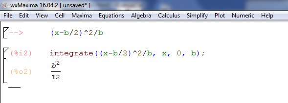
And we can go back to simpy to get the analytical form: copy and paste integrate((x-b/2)^2/b,(x,0,b)), or use wxMaxima to find that the variance is b2/12. And here's wxMaxima:
One really nice thing about wxMaxima is that you can export the results as text that R will understand. For example, here are the partial derivatives of the Gompertz survival function:
If the Gompertz survivorship is written as:
exp(a/b*(1-exp(b*t)))
Then the partial derivative with respect to b is:
(-(a*t*exp(b*t))/b-(a*(1-exp(b*t)))/b^2)*exp((a*(1-exp(b*t)))/b)
and with respect to a is:
((1-exp(b*t))*exp((a*(1-exp(b*t)))/b))/b
But let's get back to the uniform pdf. The information above suggests some "fun with numbers" to make an inefficient standard random normal deviate generator.
my.rnorm = function (N=25000)
{
set.seed(123456)
z=vector()
for(i in 1:N) z[i]=sum(runif(12))-6
return(z)
}
z=my.rnorm()
hist(z,nc=50,pr=T); lines(seq(-4,4,.01),dnorm(seq(-4,4,.01)))
if(.Platform$OS.type=="windows") {
quartz<-function() windows()
}
quartz()
plot(density(z)); lines(seq(-4,4,.01),dnorm(seq(-4,4,.01)),col='red')
if(.Platform$OS.type=="windows") {
quartz<-function() windows()
}
quartz()
plot(ecdf(z)); lines(seq(-4,4,.01),pnorm(seq(-4,4,.01)),col='red')
So are a (probability) density and a probability the same thing? Well, first, what is a probability? There is both the frequency definition (as one uses for allele frequencies) and the subjective definition as one uses in transmission genetics, but either way probabilities are bounded by 0.0 and 1.0 (inclusive). But probability densities can be greater than 1.0, as the requirements are that they be non-negative and integrate to 1.0 across the acceptable range.
dnorm(0)
[1] 0.3989423
dnorm(0,0,.1)
[1] 3.989423
integrate(dnorm,mean=0,sd=1,-Inf,Inf)
1 with absolute error < 9.4e-05
integrate(dnorm,mean=0,sd=.01,-Inf,Inf)
1 with absolute error < 3.1e-08
dunif(.25,0,.5)
[1] 2
And where can I find more pdfs? Try Darryl Holman's vol. 2 (reference) for mle.