R code for demography chapter from Companion to Biological Anthropology, 2nd edition, edited by Clark S. Larsen
Konigsberg, Milner, and Boldsen
June 4, 2022
The following code forms the wqx and
wlx columns from Séguy and Buchet (2013) Table 8.5 (p. 132). The
results are stored in the R object Table.
model=function ()
{
P=0.1
lnP=log(P)
lq=vector()
lq[1]=-.1799+.5559*lnP
lq[2]=-.116+1.039*lq[1]
lq[3]=-.397+1.092*lq[2]
lq[4]=-.685+.673*lq[3]
lq[5]=-.536+.595*lq[4]
lq[6]=-.136+.829*lq[5]
lq[7]=.007+.971*lq[6]
lq[8]=-.087+.894*lq[7]
lq[9]=-.055+.913*lq[8]
lq[10]=-.035+.911*lq[9]
lq[11]=-.004+.931*lq[10]
lq[12]=-.008+.898*lq[11]
lq[13]=.017+.893*lq[12]
lq[14]=-.084+.741*lq[13]
lq[15]=.000+.810*lq[14]
lq[16]=-.014+.729*lq[15]
lq[17]=.029+.790*lq[16]
qx=exp(lq)
lx=vector()
lx[1]=1.0
for(i in 2:17){lx[i]=lx[i-1]-lx[i-1]*qx[i-1]}
age=c(0,1,seq(5,75,5))
Table<<-data.frame(age,qx,lx)
}
model()
The following code simulates 500 deaths using the model Table from the previous code and stores the results in the R object “deaths” with columns “open” and “close” for opening and closing ages, and “Dx” for number of deaths in each interval. Because of set.seed(42) you will get the same numbers of deaths in each interval as in the book chapter.
sim=function ()
{
set.seed(42)
bins=c(0,rev(Table$lx))
U=runif(500)
Dx=rev(hist(U,br=bins,plot=F)$counts)
Sx=rev(cumsum(rev(Dx)))
age=c(0,1,seq(5,75,5))
open=age
close=c(age[2:17],90)
deaths=data.frame(open,close,Dx)
deaths<<-deaths
}
sim()
The following code reproduces Table 13.1, the stationary life table from the 500 deaths simulated in the above code.
Tab13.1=function (dat=deaths)
{
Dx=dat$Dx
open=dat$open
close=dat$close
N.age=length(Dx)
lx=vector()
lx[1]=sum(Dx)
for(i in 2:N.age) lx[i]=lx[i-1]-Dx[i-1]
qx=round(Dx/lx,4)
Lx=vector()
lx=c(lx,0)
w=close-open
mx=round(2*qx/(w*(2-qx)),4)
mid=open+w/2
for(i in 1:N.age) Lx[i]=(lx[i]+lx[i+1])/2*w[i]
Tx=rev(cumsum(rev(Lx)))
lx=lx[-(N.age+1)]
ex=round(Tx/lx[-(N.age+1)],2)
cx=round(Lx/Tx[1],4)
years=round(cx*mid,3)
LfTable=data.frame(open,close,Dx,lx,qx,Lx,mx,Tx,ex,cx,years)
print(LfTable,row.names=FALSE)
cat('\nMAL = ',round(sum(years),2),'\n')
cat('MAD = ',round(ex[1],2),'\n')
cat('b = ',round(1/ex[1],3),'\n')
cat('d = ',round(1/ex[1],3),'\n')
cat('r = 0','\n')
}

Tab13.1()
open close Dx lx qx Lx mx Tx ex cx years
0 1 115 500 0.2300 442.5 0.2599 9877.5 19.75 0.0448 0.022
1 5 65 385 0.1688 1410.0 0.0461 9435.0 24.51 0.1427 0.428
5 10 31 320 0.0969 1522.5 0.0204 8025.0 25.08 0.1541 1.156
10 15 33 289 0.1142 1362.5 0.0242 6502.5 22.50 0.1379 1.724
15 20 46 256 0.1797 1165.0 0.0395 5140.0 20.08 0.1179 2.063
20 25 41 210 0.1952 947.5 0.0433 3975.0 18.93 0.0959 2.158
25 30 31 169 0.1834 767.5 0.0404 3027.5 17.91 0.0777 2.137
30 35 23 138 0.1667 632.5 0.0364 2260.0 16.38 0.0640 2.080
35 40 27 115 0.2348 507.5 0.0532 1627.5 14.15 0.0514 1.928
40 45 27 88 0.3068 372.5 0.0725 1120.0 12.73 0.0377 1.602
45 50 20 61 0.3279 255.0 0.0784 747.5 12.25 0.0258 1.226
50 55 14 41 0.3415 170.0 0.0824 492.5 12.01 0.0172 0.903
55 60 9 27 0.3333 112.5 0.0800 322.5 11.94 0.0114 0.655
60 65 6 18 0.3333 75.0 0.0800 210.0 11.67 0.0076 0.475
65 70 3 12 0.2500 52.5 0.0571 135.0 11.25 0.0053 0.358
70 75 3 9 0.3333 37.5 0.0800 82.5 9.17 0.0038 0.276
75 90 6 6 1.0000 45.0 0.1333 45.0 7.50 0.0046 0.380
MAL = 19.57
MAD = 19.75
b = 0.051
d = 0.051
r = 0 The following code reproduces Table 13.2, the fertility schedule assuming r=0 and using the K values from Weiss (1973) Table 12 and using the methods given in his monograph.
Tab13.2=function (dat=deaths)
{
Dx=dat$Dx
N.age=length(Dx)
Dx=Dx/sum(Dx)
lx=vector()
lx[1]=1
for(i in 2:N.age) lx[i]=lx[i-1]-Dx[i-1]
open=dat$open
start=which(open==15)
lx=lx[start:(start+6)]
Age=open[start:(start+6)]
Lx=vector()
lx=c(lx,0)
for(i in 1:7) Lx[i]=(lx[i]+lx[i+1])/2*5
lx=lx[-8]
Kx=c(0.64199,1.73859,1.74068,1.41042,0.98137,0.40670,0.08418)
KxLx=Kx*Lx
aveb=1/sum(KxLx)
FB=Kx*aveb
TFR=sum(FB)*5
LxFB=Lx*FB
Years=LxFB*(Age+2.5)
T=sum(Years)
KxLx=round(KxLx,3)
FB=round(FB,3)
LxFB=round(LxFB,3)
Years=round(Years,2)
LfTable=data.frame(Age,lx,Lx,Kx,KxLx,FB,LxFB,Years)
print(LfTable,row.names=FALSE)
cat('\nTFR = ',round(TFR,2),'\n')
cat('T = ',round(T,2),'\n')
}


Tab13.2()
Age lx Lx Kx KxLx FB LxFB Years
15 0.512 2.330 0.64199 1.496 0.061 0.141 2.48
20 0.420 1.895 1.73859 3.295 0.164 0.312 7.01
25 0.338 1.535 1.74068 2.672 0.165 0.253 6.95
30 0.276 1.265 1.41042 1.784 0.133 0.169 5.49
35 0.230 1.015 0.98137 0.996 0.093 0.094 3.53
40 0.176 0.745 0.40670 0.303 0.038 0.029 1.22
45 0.122 0.305 0.08418 0.026 0.008 0.002 0.12
TFR = 3.31
T = 26.79 The code below reproduces Table 13.3 (a life table with r=0.02) from the chapter. The method follows Table 5 from Asch (1976).
Tab13.3=function (r=0.02)
{
Dx=deaths$Dx
open=deaths$open
close=deaths$close
w=close-open
mid=open+w/2
e.ra=exp(r*mid)
N.age=length(Dx)
adj.Dx=e.ra*Dx
lx=vector()
lx[1]=sum(adj.Dx)
for(i in 2:N.age) lx[i]=lx[i-1]-adj.Dx[i-1]
Lx=vector()
lx=c(lx,0)
for(i in 1:N.age) Lx[i]=(lx[i]+lx[i+1])/2*w[i]
Tx=rev(cumsum(rev(Lx)))
lx=lx[-(N.age+1)]
ex=round(Tx/lx[-(N.age+1)],2)
adj.Lx=Lx/e.ra
sum.adj.Lx=sum(adj.Lx)
b=sum(adj.Dx)/sum.adj.Lx
cx=adj.Lx/sum.adj.Lx
Lx=round(Lx,1)
Tx=round(Tx,1)
adj.Lx=round(adj.Lx,2)
years=cx*mid
MAL=sum(years)
d=b-r
MAD=(1-r*MAL)/d
years=round(years,3)
e.ra=round(e.ra,3)
lx=round(lx,2)
cx=round(cx,4)
adj.Dx=round(adj.Dx,2)
LfTable=data.frame(open,close,Dx,e.ra,adj.Dx,lx,Lx,Tx,ex,adj.Lx,cx,years)
print(LfTable,row.names=FALSE)
cat('\nMAL =',round(MAL,2))
cat('\nMAD =',round(MAD,2))
cat('\nb =',round(b,3))
cat('\nd =',round(d,3))
cat('\nr =',r,'\n')
}
Tab13.3()
open close Dx e.ra adj.Dx lx Lx Tx ex adj.Lx cx years
0 1 115 1.010 116.16 807.95 749.9 23177.6 28.69 742.41 0.0483 0.024
1 5 65 1.062 69.02 691.80 2629.1 22427.7 32.42 2476.03 0.1611 0.483
5 10 31 1.162 36.02 622.78 3023.8 19798.5 31.79 2602.64 0.1694 1.270
10 15 33 1.284 42.37 586.76 2827.9 16774.7 28.59 2202.34 0.1433 1.792
15 20 46 1.419 65.28 544.39 2558.7 13946.8 25.62 1803.11 0.1173 2.054
20 25 41 1.568 64.30 479.11 2234.8 11388.1 23.77 1424.97 0.0927 2.087
25 30 31 1.733 53.73 414.81 1939.7 9153.3 22.07 1119.12 0.0728 2.003
30 35 23 1.916 44.06 361.08 1695.2 7213.6 19.98 884.99 0.0576 1.872
35 40 27 2.117 57.16 317.02 1442.2 5518.4 17.41 681.25 0.0443 1.663
40 45 27 2.340 63.17 259.86 1141.4 4076.2 15.69 487.84 0.0317 1.349
45 50 20 2.586 51.71 196.69 854.2 2934.8 14.92 330.34 0.0215 1.021
50 55 14 2.858 40.01 144.98 624.9 2080.6 14.35 218.66 0.0142 0.747
55 60 9 3.158 28.42 104.97 453.8 1455.7 13.87 143.69 0.0094 0.538
60 65 6 3.490 20.94 76.55 330.4 1002.0 13.09 94.65 0.0062 0.385
65 70 3 3.857 11.57 55.60 249.1 671.6 12.08 64.57 0.0042 0.284
70 75 3 4.263 12.79 44.03 188.2 422.5 9.60 44.14 0.0029 0.208
75 90 6 5.207 31.24 31.24 234.3 234.3 7.50 45.00 0.0029 0.242
MAL = 18.02
MAD = 19.63
b = 0.053
d = 0.033
r = 0.02 This code produces Figure 13.1A, a Brass (1971) 2-parameter logit model and a Ewbank, Leon, and Stoto (1983) 4-parameter logit model fit to the simulated death data.
Brass=structure(c(1, 2, 3, 4, 5, 6, 7, 8, 9, 10, 11, 12, 13, 14, 15,
16, 17, 18, 19, 20, 21, 22, 23, 24, 25, 26, 27, 28, 29, 30, 31,
32, 33, 34, 35, 36, 37, 38, 39, 40, 41, 42, 43, 44, 45, 46, 47,
48, 49, 50, 52.5, 55, 57.5, 60, 62.5, 65, 67.5, 70, 72.5, 75,
77.5, 80, 82.5, 85, 87.5, 90, 92.5, 95, 97.5, 0.8499, 0.807,
0.7876, 0.7762, 0.7691, 0.7642, 0.7601, 0.7564, 0.7532, 0.7502,
0.7477, 0.7452, 0.7425, 0.7396, 0.7362, 0.7328, 0.7287, 0.7241,
0.7188, 0.713, 0.7069, 0.7005, 0.6943, 0.6884, 0.6826, 0.6764,
0.6703, 0.6643, 0.6584, 0.6525, 0.6466, 0.6405, 0.6345, 0.6284,
0.6223, 0.616, 0.6097, 0.6032, 0.5966, 0.5898, 0.583, 0.5759,
0.5686, 0.5612, 0.5535, 0.5454, 0.5371, 0.5285, 0.5197, 0.5106,
0.4857, 0.4585, 0.4291, 0.3965, 0.3602, 0.321, 0.2801, 0.238,
0.1945, 0.15, 0.109, 0.076, 0.049, 0.029, 0.0155, 0.007, 0.003,
0.001, 1e-04), .Dim = c(69L, 2L))

four.parm=function (K=.01,L=.01,dat=deaths)
{

# Reference survivorship from Ewbank et al. 1983 under 15 combined with
# Brass 1971 from 15 and older
l.s=c(0.842, .80834,.79108,.78004,.77208,.74883)
age=c(1,2,3,4,5,10)
ref=matrix(rbind(cbind(age,l.s),Brass[-(1:14),]),nc=2)

# Survivorship from simulated life table
Dx=dat$Dx
N=sum(Dx)
Sx=rev(cumsum(rev(Dx)))
lx=(Sx/N)[-1]

age=dat$open[-1]
l.s=ref[ref[,1] %in% age,2]
N.age=length(lx)

yx=0.5*log(lx/(1-lx))

T=function(p,K,L)
{
if(p<0.5){
   sto=1-((1-p)/p)^L
   return(sto/(2*L))
}
sto=p/(1-p)
sto=sto^K-1
return(sto/(2*K))
}

leastSQ=function(x)
{
a=x[1]
b=x[2]
K=x[3]
L=x[4]
TKL=vector()
LS=0
for(i in 1:N.age){
  TKL[i]=T(l.s[i],K,L)
  LS=LS+(yx[i]-(a+b*TKL[i]))^2
}
return(LS)
}

x=c(0,1,.1,.1)
x=optim(x,leastSQ)$par
K=x[3]
L=x[4]
TKL=vector()
for(i in 1:N.age){
  TKL[i]=T(l.s[i],K,L)
}

ab=coef(lm(yx~TKL))

N.age=NROW(ref)
TKL2=vector()
for(i in 1:N.age){
  TKL2[i]=T(ref[i,2],K,L)
}


pred.lx=ab[1]+ab[2]*TKL2
pred.lx=exp(2*pred.lx)/(1+exp(2*pred.lx))
lines(c(0,ref[,1]),c(1,pred.lx))
}


fit.brass=function (dat=deaths)
{
# Brass 1971 reference survivorship
age=dat$open[-1]
l.s=Brass[Brass[,1] %in% age,2]

# Survivorship from simulated life table
Dx=dat$Dx
N=sum(Dx)
Sx=rev(cumsum(rev(Dx)))
l.x=(Sx/N)[-1]
yx=log((1-l.x)/l.x)
ys=log((1-l.s)/l.s)
l.s=Brass[,2]
l.s=log((1-l.s)/l.s)
ab=coef(lm(yx~ys))
yb=ab[1]+ab[2]*l.s
pred.lx=1/(1+exp(yb))
plot(dat$open,c(1,l.x),pch=19,xlab='Age',ylab=expression(l[x]))
lines(c(0,Brass[,1]),c(1,pred.lx),lty=2)
}


Fig13.1A=function (dat=deaths)
{
fit.brass(dat=dat)
four.parm(dat=dat)
legend(x='topright',bty='n',legend=c('4-parameter logit','2-parameter logit'),
lty=c(1,2))
}

Fig13.1A()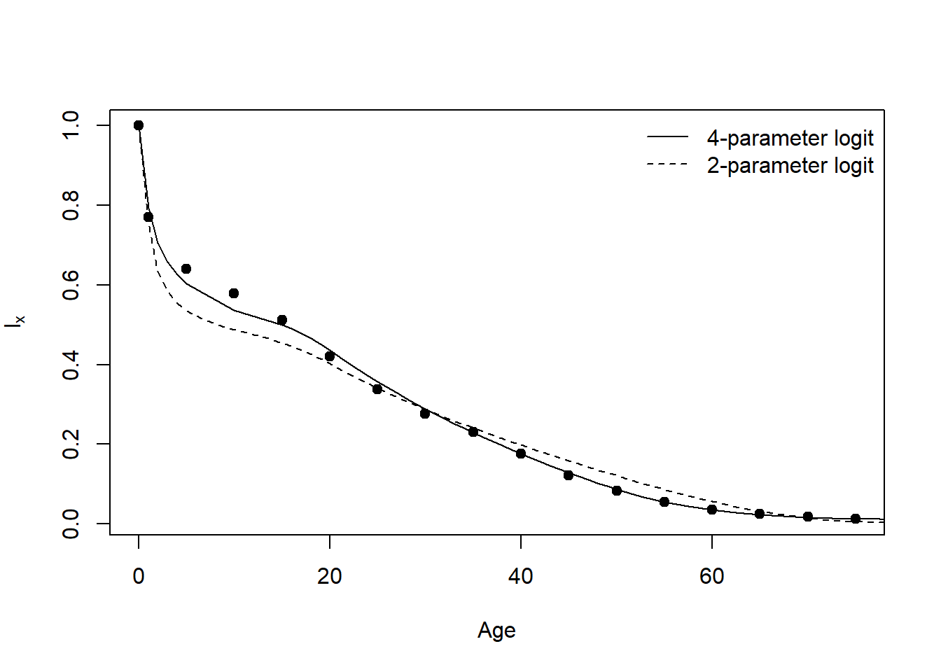
This draws Figure 13.1B, a Gompertz (1825) hazard fit to the simulated data and drawn as survivorship. The points are the survivorship from the life table. Note that the hazard starts at age 15, so the survivorship at that age is 1.0. Also note that you will need the R package “alabama” to run this code.
Fig13.1B=function ()
{
library(alabama)
dat=deaths$Dx[-(1:4)]
N=sum(dat)
lx=rev(cumsum(rev(dat))/N)
age=seq(15,75,5)
plot(age,lx,pch=19,xlab='Age',ylab=expression(l[x]))
dat=matrix(cbind(age,dat),nc=2)
open=vector()
close=vector()
for(i in 1:13){
   open[i]=dat[i,1]-15
   close[i]=open[i]+5
}

S=function(x,t){
a=x[1]
b=x[2]
return(exp(a/b*(1-exp(b*t))))
}
x=c(0.05, 0.02)

lnLK=function(x){
  zloglik=0
  for(i in 1:12){
    zloglik=zloglik+dat[i,2]*log(S(x,open[i])-S(x,close[i]))
 }
 zloglik=zloglik+dat[13,2]*log(S(x,dat[13,1]-15))
 return(as.numeric(zloglik))
}

hin = function(x) {
h = vector()
h[1] = x[1]
h[2] = x[2]
h
}

x=constrOptim.nl(par=x,lnLK,hin=hin,control.optim = list(fnscale=-1))$par
age=15:75
lines(age,S(x,age-15))

}

Fig13.1B()
Loading required package: numDeriv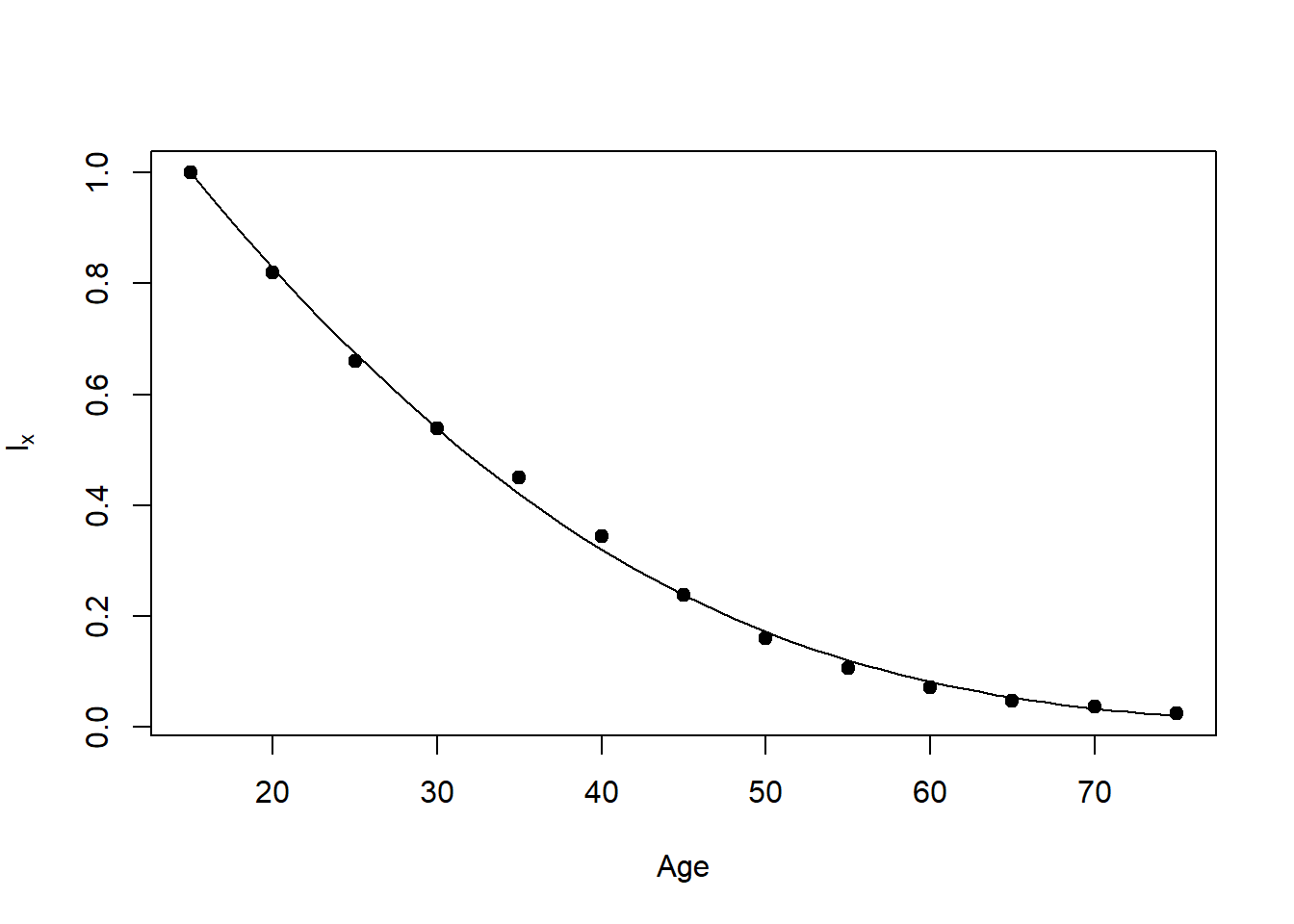
Min(hin):  0.02
par:  0.05 0.02
fval:  -611.4845
Min(hin):  0.01837235
par:  0.03590705 0.01837235
fval:  -593.0168
Min(hin):  0.01837235
par:  0.03590705 0.01837235
fval:  -593.0168
The following code fits a Siler (1979) model without the constant, a2 parameter, and draws it as survivorship. Again, you will need the R package “alabama”.
Fig13.1C=function ()
{
library(alabama)

dat=deaths
Dx=dat[,3]
lx=rev(cumsum(rev(Dx)))/sum(Dx)
Age=deaths$open
plot(Age,lx,pch=19,ylab=expression(l[x]))

S=function(x,a){
  a1=x[1]
  b1=x[2]
  a3=x[3]
  b3=x[4]
  neg.Gomp=-a1/b1*(1-exp(-b1*a))
  Gomp=a3/b3*(1-exp(b3*a))
  return(exp(neg.Gomp+Gomp))
}


lnLK=function(x){
  zloglik=0
  S.val=vector()
  for(i in 1:17){
     S.val=S(x,dat[,1])
  }
  S.val[18]=0
  for(i in 1:17){
    zloglik=zloglik+dat[i,3]*log(S.val[i]-S.val[i+1])
  }
return(zloglik)
}

hin = function(x) {
h = vector()
h[1] = x[1]
h[2] = x[2]
h[3] = x[3]
h[4] = x[4]
h
}

x=c(0.4, 1.25, 0.02, 0.02)

x=constrOptim.nl(par=x,lnLK,hin=hin,control.optim = list(fnscale=-1))$par

haz=function(a){
a1=x[1]
b1=x[2]
a3=x[3]
b3=x[4]
ft=a1*exp(-b1*a)+a3*exp(b3*a)
return(ft)
}

surv=function(a){
a1=x[1]
b1=x[2]
a3=x[3]
b3=x[4]
St=exp(-a1/b1*(1-exp(-b1*a))+a3/b3*(1-exp(b3*a)))
return(St)
}

Age=0:75
lines(Age,surv(Age))
return()

ft=function(a) {haz(a)*surv(a)*a}

integrate(Vectorize(ft),lower=0,upper=100)

}
Fig13.1C()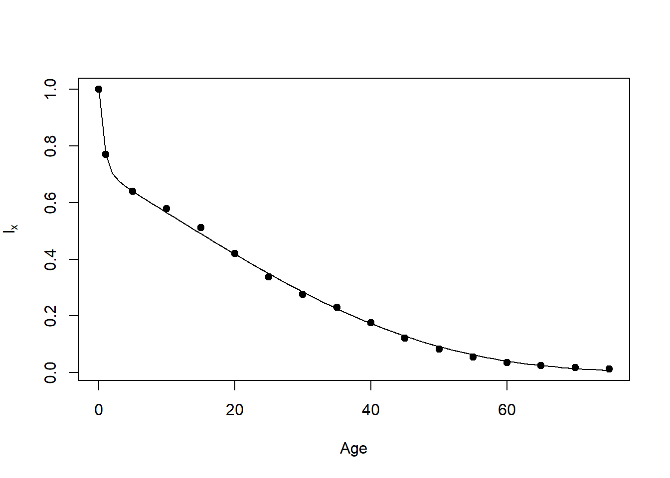
Min(hin):  0.02
par:  0.4 1.25 0.02 0.02
fval:  -1249.953
Min(hin):  0.0206569
par:  0.422762 1.256735 0.0206569 0.02483714
fval:  -1244.389
Min(hin):  0.0206569
par:  0.422762 1.256735 0.0206569 0.02483714
fval: -1244.389 NULLThe following code produces Figure 13.1D, a mixed Makeham model (Wood et al. 2002), but where high risk individuals follow a Makeham mortality model and low risk individuals follow a Gompertz mortality model.
Fig.13.1D=function ()
{
library(alabama)

dat=deaths
Dx=dat[,3]
lx=rev(cumsum(rev(Dx)))/sum(Dx)
Age=deaths$open
plot(Age,lx,pch=19,ylab=expression(l[x]))

S=function(x,a){
  p=x[1]
  a1=x[2]
  a3=x[3]
  b3=x[4]
  S1=p*exp(-a1*a+a3/b3*(1-exp(b3*a)))
  S2=(1-p)*exp(a3/b3*(1-exp(b3*a)))
  return(S1+S2)
}

lnLK=function(x){
  zloglik=0
  S.val=vector()
  for(i in 1:17){
     S.val=S(x,dat[,1])
  }
  S.val[18]=0
  for(i in 1:17){
    zloglik=zloglik+dat[i,3]*log(S.val[i]-S.val[i+1])
  }
return(zloglik)
}


hin = function(x) {
h = vector()
h[1] = x[1]
h[2] = 1-x[1]
h[3] = x[2]
h[4] = x[3]
h[5] = x[4]
h
}

x=c(0.5, 1.5, 0.005, 0.05)

x=constrOptim.nl(par=x,lnLK,hin=hin,control.optim = list(fnscale=-1))$par
print(round(x,4))

surv=function(a){
  p=x[1]
  a1=x[2]
  a3=x[3]
  b3=x[4]
  S1=p*exp(-a1*a+a3/b3*(1-exp(b3*a)))
  S2=(1-p)*exp(a3/b3*(1-exp(b3*a)))
  return(S1+S2)
}

Age=0:75
lines(Age,surv(Age))
}

Fig.13.1D()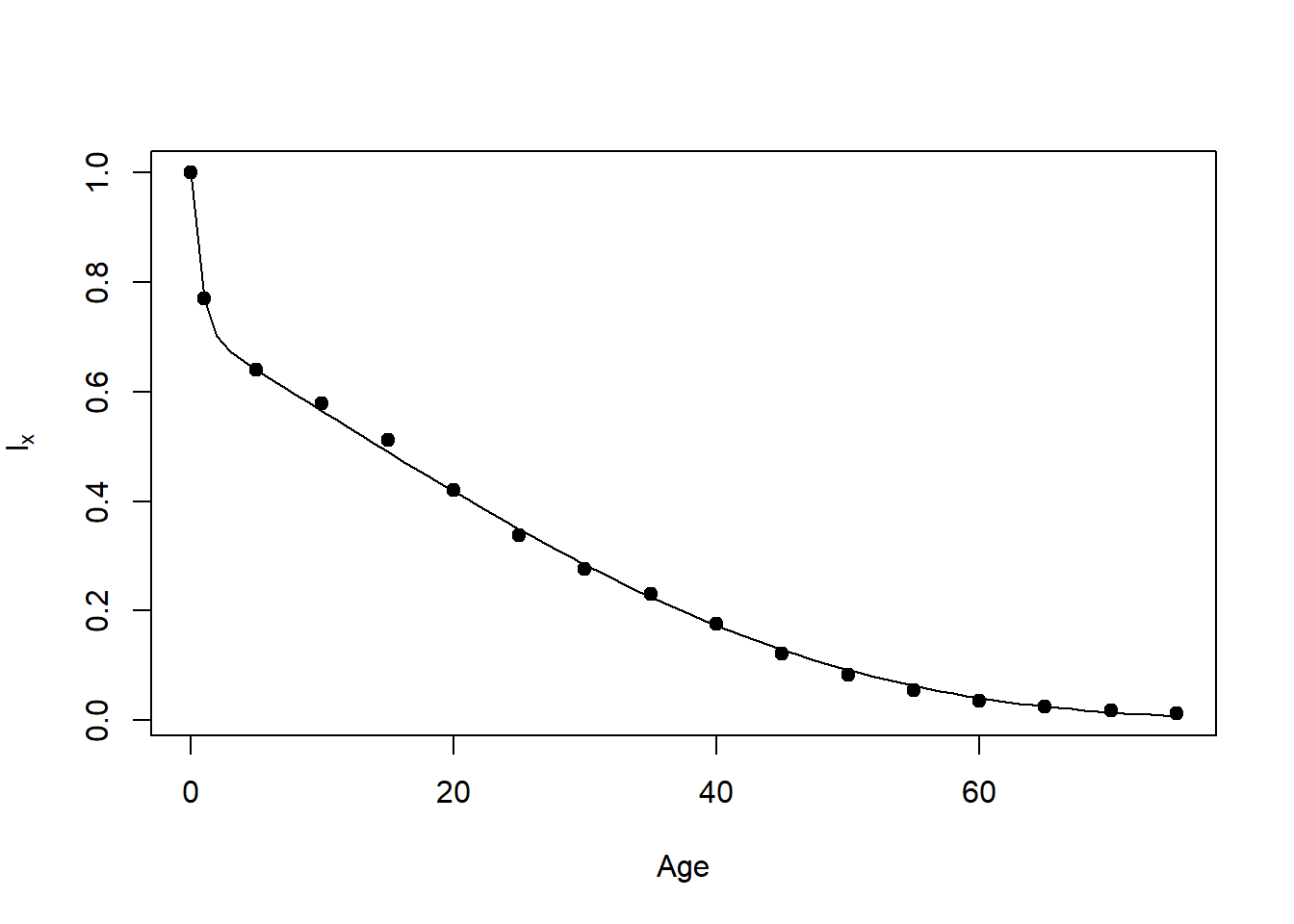
Min(hin):  0.005
par:  0.5 1.5 0.005 0.05
fval:  -1350.155
Min(hin):  0.02071649
par:  0.2856456 1.380901 0.02071649 0.02478278
fval:  -1244.375
[1] 0.2856 1.3809 0.0207 0.0248
The following code extracts the crude birth rate, crude death rate, mean age in the living, and mean age in the dead after fitting a Siler model without the a2 parameter. The first run is with r=0 (stationary).
haz.parms=function (r=0.02,dat=deaths)
{
library(alabama)

# Adjust deaths by exp(r*a) where r=growth rate & a=mid-point age
mid.age=(dat[,1]+dat[,2])/2
Dx=dat[,3]*exp(r*mid.age)
N.age=length(Dx)

S=function(x,a){
  a1=x[1]
  b1=x[2]
  a3=x[3]
  b3=x[4]
  neg.Gomp=-a1/b1*(1-exp(-b1*a))
  Gomp=a3/b3*(1-exp(b3*a))
  return(exp(neg.Gomp+Gomp))
}

lnLK=function(x){
  zloglik=0
  S.val=vector()
  for(i in 1:N.age){
     S.val=S(x,dat[,1])
  }
  S.val[N.age+1]=0
  for(i in 1:N.age){
    zloglik=zloglik+ Dx[i]*log(S.val[i]-S.val[i+1])
  }
return(zloglik)
}

hin = function(x) {
h = vector()
h[1] = x[1]
h[2] = x[2]
h[3] = x[3]
h[4] = x[4]
h
}

x=c(0.4, 1.25, 0.02, 0.02)

x=constrOptim.nl(par=x,lnLK,hin=hin,control.optim = list(fnscale=-1))$par

haz=function(a){
a1=x[1]
b1=x[2]
a3=x[3]
b3=x[4]
ft=a1*exp(-b1*a)+a3*exp(b3*a)
return(ft)
}

surv=function(a){
a1=x[1]
b1=x[2]
a3=x[3]
b3=x[4]
St=exp(-a1/b1*(1-exp(-b1*a))+a3/b3*(1-exp(b3*a)))
return(St)
}

ft=function(a) {haz(a)*surv(a)}
denom=function(a) {exp(-r*a)*ft(a)}
num=function(a) {a*denom(a)}

x=constrOptim.nl(par=x,lnLK,hin=hin,control.optim = list(fnscale=-1))$par
inv.b=function(a) {surv(a)*exp(-r*a)}

denom.b=integrate(Vectorize(inv.b),lower=0,upper=120)$val
b=1/denom.b
cat('\nb =',round(b,3))

d=function(a) {exp(-r*a)*ft(a)}

cat('\nd =',round(integrate(d,lower=0,upper=120)$val/denom.b,3))
cat('\nr =',r)

get.MAL = function(a) {a*exp(-r*a)*surv(a)}

MAL=b*integrate(Vectorize(get.MAL),lower=0,upper=120)$val
cat('\nMAL =',round(MAL,2))

MAD=integrate(Vectorize(num),lower=0,upper=120)$val /
    integrate(Vectorize(denom),lower=0,upper=120)$val
cat('\nMAD =',round(MAD,2),'\n')

}


haz.parms(r=0)
Min(hin): 0.02
par: 0.4 1.25 0.02 0.02
fval: -1249.953
Min(hin): 0.0206569
par: 0.422762 1.256735 0.0206569 0.02483714
fval: -1244.389
Min(hin): 0.0206569
par: 0.422762 1.256735 0.0206569 0.02483714
fval: -1244.389
Min(hin): 0.0206569
par: 0.422762 1.256735 0.0206569 0.02483714
fval: -1244.389
b = 0.051
d = 0.051
r = 0
MAL = 19.68
MAD = 19.59 And now with the default value of r=0.02.
haz.parms()Min(hin): 0.02
par: 0.4 1.25 0.02 0.02
fval: -2236.772
Min(hin): 0.01303957
par: 0.2605069 1.368529 0.01303957 0.02791064
fval: -2196.292
Min(hin): 0.01303957
par: 0.2605069 1.368529 0.01303957 0.02791064
fval: -2196.292
Min(hin): 0.01303957
par: 0.2605069 1.368529 0.01303957 0.02791064
fval: -2196.292
Min(hin): 0.01303957
par: 0.2605069 1.368529 0.01303957 0.02791064
fval: -2196.292
b = 0.053
d = 0.033
r = 0.02
MAL = 18.15
MAD = 19.3