Most Likely Number of Individuals (MLNI)
Excel Spreadsheet 1 – For a single element
Excel Spreadsheet 2 – For multiple elements (4 in this case)
The above links will download Excel spreadsheets with MLNI calculations. You can edit the blue numbers to put in different bone counts.
“R” Script for
finding “highest density regions” (HDRs)
This section uses “R,” which you can obtain from http://cran.r-project.org/. You will also need to download the supplemental library “SuppDists” (see http://cran.r-project.org/doc/packages/SuppDists.pdf, and the simplest way to get this is to install “R”, then from the toolbar select “Packages” and then “Install package(s) from CRAN…”, then pick “SuppDists” from the list).
First let’s do an example for a single element, where the counts are 21 lefts, 15 rights, and 11 pairs. We make the object “bones” as follows (mark the text below, paste into the “Rgui” and hit return):
bones<-t(c(21,15,11))
Then mark the following text (between the horizontal lines), copy and paste into the Rgui:
MLNI = function (b=bones,iters=50,which=0,hdr=0)
{
library(SuppDists)
if(which>0){b<-t(b[which,])}
p<-0
p.prod<-0
lb<-NROW(b)

# Get MNI & estimated recovery rate

MNI=0
r=0
r.se=0
for(i in 1:lb){
   L=b[i,1]
   R=b[i,2]
   P=b[i,3]
   if(L+R-P>MNI){MNI=L+R-P}
   r[i]=2*P/(L+R)
   r.se[i]=sqrt((r[i]-1)^2*(r[i]-2)^2*r[i]^2/
      (r[i]^2*(L+R)*(3-2*r[i])+2*P*(2-6*r[i]+3*r[i]^2)))
}

# Get probabilities for each value of N

for(N in MNI:(MNI+iters)){
for(i in 1:lb)
 {
   L<-b[i,1]
   R<-b[i,2]
   P<-b[i,3]
   p[i]<-dghyper(P,L,R,N)*P/(N+1)
 }
p.prod[N-MNI+1]<-prod(p)
}
tot<-sum(p.prod)
p.norm<-p.prod/tot
sto<-matrix(rep(0,3*iters),nc=3)
perc<-0

# Find HDRs

for(i in 1:iters)
{
logic<-p.norm>=p.norm[i]
nhi<-sum(logic)
lo<-which.max(logic)
hi<-lo+nhi-1
perc<-round(sum(p.norm[p.norm>=p.norm[i]])*100,1)
sto[i,]<-c(perc,lo+MNI-1,hi+MNI-1)
}
sto<-sto[1:(i-1),]
ix<-sort(sto[,1],decreasing=T,index.return=T)$ix
sto<-sto[ix,]
plot(c(rep((MNI):(MNI+iters),each=2),MNI+iters),c(0,rep(p.norm,each=2)),
type="l",xlab='N',ylab='Probability',xlim=c(sto[1,2],sto[1,3]+1))
lines(c(sto[1,2],sto[1,3]),c(0,0))
print(sto)
print(cbind(r,r.se))
if(hdr==0){return(cat('Run again with hdr= row for plot of hdr\n'))}
lo<-sto[hdr,2]
hi<-sto[hdr,3]+1
if(lo==MNI){polygon(c(rep(lo:hi,each=2)),c(0,rep(p.norm[(lo-MNI):(hi-MNI)],each=2),0),density=10)}
if(lo>MNI){polygon(c(rep(lo:hi,each=2)),c(0,rep(p.norm[(lo-MNI+1):(hi-MNI)],each=2),0),density=10)}
mtext(paste(sto[hdr,1],'% HDR',sep=''),line=1,cex=1.5)
}
NOTE (added Jan 22, 2005) – A number of people have
noted that this script did not work when counts were very high (like L = 250, R
= 300, and P = 200) or if there were multiple elements that gave conflicting
results. I have fixed this problem
today, but be forewarned that the script will now sometimes return multiple
“100% HDRs.” If you see this take the
narrowest interval as the 100%. Also be
forewarned that you are responsible for setting “iters” to whatever value is
necessary.
NOTE (added Sep 4, 2012) - Calculation of recovery rates and standard error added
Now at the prompt in the Rgui type:
MLNI()
And you will see the following:
[,1] [,2] [,3][1,] 100.0 25 60
[2,] 99.9 25 54
[3,] 99.9 25 55
[4,] 99.9 25 56
[5,] 99.9 25 57
[6,] 99.9 25 58
[7,] 99.9 25 59
[8,] 99.8 25 52
[9,] 99.8 25 53
[10,] 99.7 25 50
[11,] 99.7 25 51
[12,] 99.6 25 49
[13,] 99.5 25 48
[14,] 99.4 25 47
[15,] 99.2 25 46
[16,] 99.0 25 45
[17,] 98.7 25 44
[18,] 98.4 25 43
[19,] 98.0 25 42
[20,] 97.4 25 41
[21,] 96.7 25 40
[22,] 95.8 25 39
[23,] 94.6 25 38
[24,] 93.1 25 37
[25,] 91.1 25 36
[26,] 88.5 25 35
[27,] 85.2 25 34
[28,] 80.9 25 33
[29,] 76.4 26 33
[30,] 70.9 26 32
[31,] 64.1 26 31
[32,] 55.6 26 30
[33,] 46.3 27 30
[34,] 36.1 27 29
[35,] 24.5 27 28
[36,] 12.5 28 28
Run again with hdr= row for plot of hdr
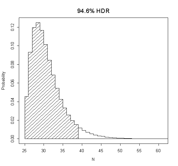
This matrix is telling you about the various HDRs. The first column gives the percentage for the HDR, while the second and third columns give the HDR (inclusive). For example, on the 23rd row (marked with [23,]) the 94.6% HDR is given which runs from 25 to 38. If you want to plot this specific HDR then run again as:
MLNI(hdr=23)
which produces the following plot:
Now try an example with multiple elements. Mark, copy and paste the following:
bones<-matrix(c(9,9,6,7,7,4,7,9,3),nc=3,byrow=T)
and run as before. Note that if you only want to run this for one of the three elements then the format is:
MLNI(which=2)
Where your are specifying the second element and then, say:
MLNI(which=2,hdr=32)
Derivation of Chapman’s estimator
Using results from Roberts (1967: eqn 2.11, and see also Lee [1997:200-202]), we write the probability of N conditional on L, R, and P as:
 (1)
(1)
where
![]() is the probability
from the hypergeometric distribution of getting P pairs, upon drawing L
lefts and R rights from N individuals. To find the maximum likelihood estimator from equation (1) write
the ratio of adjacent probabilities as:
is the probability
from the hypergeometric distribution of getting P pairs, upon drawing L
lefts and R rights from N individuals. To find the maximum likelihood estimator from equation (1) write
the ratio of adjacent probabilities as:
 (2)
(2)
For values of N less than the maximum likelihood estimate this ratio will be greater than one, while for values of N greater than the maximum likelihood estimate this ratio will be less than one. Solve the inequality:
![]() (3)
(3)
to find that the maximum likelihood estimate occurs at:

which is Chapman’s estimator.
Estimating the recovery
probability
Instead of estimating N it may be desirable to estimate the “recovery probability,” or “r.” The recovery probability (r) is defined here as the probability that a bone will make its way into the sample being analyzed. Assuming that the probability of recovering a left bone is equal to that of recovering a right, the maximum likelihood estimate of r is:
![]() (4)
(4)
and the asymptotic standard error of the estimate is:
 (5)
(5)
LITERATURE CITED
Chapman DG. 1951. Some properties of the hypergeometric distribution with applications to zoological sample census. University of California Publications in Statistics 1:131-159.
Lee PM. 1997. Bayesian statistics: an introduction, 2nd ed. New York: Oxford University Press.
Roberts
HV. 1967. Informative stopping rules and inference about population size. J Am Statist Assoc 62:763-775.
