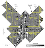
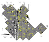
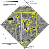
Dr. Michael L. Hargrave (ERDC CERL) conducted geophysical surveys at the New Philadelphia site, Pike County, Illinois, during visits in: April, May, and June of 2004; May and June of 2005; and March, May and June of 2006. The objectives of this work were to identify subsurface archaeological features associated with 19th century occupation of the site, and to provide field school students with an introduction to the use of geophysical survey in archaeological field research. The geophysical work was conducted in support of the ongoing, NSF-funded field school and related investigations at the New Philadelphia site conducted by the University of Maryland, Illinois State Museum, University of Illinois, and the New Philadelphia Association.

Archaeological features such as pits, privies, cisterns, domestic architecture, etc., represent localized disturbances to soils that would otherwise comprise relatively homogeneous deposits (at the spatial scale relevant to archaeological sites). Features frequently contain organically enriched fill that is darker in color or different in texture than the surrounding soils. It is often this visual (and, to some extent, textural) contrast that permits archaeologists to detect features during excavation. Similarly, geophysical techniques can detect subsurface archaeological features that contrast with the surrounding soils in terms of electrical resistance, magnetic, or other properties. Factors that can create a geophysical contrast include soil compaction, particle size, organic content, artifact content, burning, and moisture retention. Remnant magnetism and magnetic susceptibility are particularly relevant for magnetic feature detection. Heating iron oxides (present in many soils) above ca. 400 degrees Centigrade results in a permanent change (remnant magnetism) in the object’s magnetic field. Human occupation often introduces burned and organic materials to the local soils and increases magnetic susceptibility. In general, any human action that involves the localized disturbance of the soil is potentially detectable by geophysical techniques. Localized disturbances associated with tree roots, rodents, and other natural phenomena, as well as recent cultural activities (vehicle ruts, plow furrows, etc.) are also often detectable.

In a geophysical map, cultural features (as well as other discrete disturbances) may appear as anomalies, i.e., spatially discrete areas characterized by geophysical values that differ from those of the surrounding area. Prehistoric features such as pits and hearths are typically characterized by a very low contrast with the surrounding soil matrix. Historic features frequently contain metal artifacts and architectural debris (brick, mortar, stone footings, etc.) and thus typically exhibit a stronger contrast with their surroundings.

Several other factors can make it difficult to identify anomalies associated with low contrast features. All geophysical surveys are to some extent affected by noise, a seemingly random component in the data attributable to the instrument itself, the operator’s field technique, or variability in the site’s soil, rocks, etc. Clutter refers to non-archaeological, non-random, discrete phenomena that complicate feature detection. Clutter can include plow furrows, rocks, tree roots, rodent burrows, and modern metallic debris. At some sites, anomalies associated with clutter can be stronger and more numerous than anomalies related to cultural features.

Two geophysical techniques were used at the New Philadelphia Site: magnetic field gradiometry and electrical resistance. The magnetic survey (Bevan 1998; Heimmer and De Vore 1995; Scollar 1990) was conducted using a Geoscan FM36 gradiometer. This instrument is manufactured by Geoscan Research, a small firm in Great Britain that produces geophysical instruments and software optimized for archaeological applications. The gradiometer can measure exceedingly subtle disruptions in the earth's magnetic field that were caused by prehistoric and historic-era cultural activities, as well as recent cultural and natural phenomena.

The Geoscan FM36 records the difference or gradient between the values measured by two fluxgate sensors that are positioned at slightly different (.5 meter) distances from the ground surface. To collect data, the surveyor walks along a predefined transect, carrying the gradiometer in one hand. A sound emitted by the instrument's automatic trigger allows the surveyor to distribute the data collection points at regular intervals. The surveyor must take care to keep the tube containing the two magnetic sensors perpendicular to the ground surface. Deviations of the instrument from the perpendicular are manifested in the data as slightly anomalous readings. The overall effect of such anomalous values is to decrease the signal to noise ratio, making it less likely that very subtle features will be detected.

In preparation for the survey, a metric grid comprised of 20 by 20 meter blocks was established at the site. Blocks of this size represent a widely used data collection unit for many geophysical studies, particularly those conducted using Geoscan instruments. The blocks were oriented approximately 45 degrees east of magnetic north. This deviation from the New Philadelphia historic town plat (which is oriented to the cardinal directions) was necessary to prevent the obfuscation of linear features as a result of magnetic processing techniques (the zero mean traverse routine in Geoplot software can remove linear features that are parallel to the data collection traverses).

In each block, the survey began in the west corner and proceeded northeast and southwest along transects that were spaced at 1 meter intervals. Transects were marked using nonmagnetic tapes held in place by plastic tent pegs. The gradiometer was set for its maximum resolution (.1 nanoTesla). The survey area was in tall (ca. 20 cm) grass and field conditions were generally favorable.

In the gradiometer surveys, data values were collected at .125 m intervals as the surveyor moved along each transect. This strategy resulted in a medium-density survey (8 data values per square meter) and reasonably high-resolution maps.

Resistance surveys (Bevan 1998; Hargrave et al. 2002; Heimmer and De Vore 1995; Scollar 1990) introduce an electrical current into the ground and measure the ease or difficulty with which the current (measured in ohms) flows through the soil. Cultural features and other localized soil disturbances can be detected if they differ sufficiently from the surrounding soil in terms of their resistance to the passage of the current. The number and mobility of free charge carriers (principally soluble ions) are the primary determinants of electrical resistance. The simultaneous availability of soil moisture and soluble salts determines the free charge carrier concentration in the soil. The mobility of the soluble ions is governed by soil moisture content, soil grain size, temperature, soil compaction, and the surface chemistry of the soil grains (Somers and Hargrave 2001). In situations where the fill of cultural features hold moisture more readily than the surrounding soils, the pits may be manifested by low resistance anomalies. Alternatively, features characterized by relatively coarse or loosely compacted (well-drained) fill may be associated with high resistance anomalies. A pit that is manifested by a high resistance anomaly in one season can conceivably be associated with a low resistance anomaly in other seasons, when relative soil moisture is different. Concentrations of building debris (bricks, stone rubble, etc.) typically exhibit relatively high resistance.

The resistance surveys at New Philadelphia were conducted using a Geoscan RM15 resistance meter equipped with a PA5 probe array and MPX multiplexer. In 2004, the instrument was configured with three probes spaced at .5 meter intervals, generally known as a parallel twin configuration. This probe spacing was selected in order to collect resistance data representative of the uppermost ca. .5 meter of deposits. This depth was selected under the assumption that features would be located immediately below the modern plow zone. In 2005 and 2006, the instrument was configured with two probes spaced at 1.0 meter width. In the resistance surveys undertaken in 2004 and 2005, data values were collected at .5 meter intervals north south along transects spaced at 1meter intervals east west. This strategy produced a relatively high-resolution survey (4 data values per square meter) that should be adequate to detect most features larger than .5 meter diameter.

The magnetic and resistance data were processed using Geoplot 3.00, a software package developed by Geoscan Research (Walker and Somers 2000) for archaeological applications. Geoplot routines were used to identify and remove data defects, detect anomalies that could be associated with cultural features, and to cosmetically improve the appearance of the maps. None of these processing steps resulted in the creation of anomalies that were not present in the raw data.

The general processing sequence for the magnetic data was as follows. Data were first Clipped to remove extreme outlying values. The Despike routine was then used to further reduce the effects of isolated data spikes. The Zero Mean Traverse routine was used to set the background mean of each traverse to zero. This removed much of the striping that is often present in the raw data. The interpolation routine was used to achieve square pixels. A Low Pass Filter was then conducted to remove high frequency, small-scale spatial detail (i.e., to smooth the data). The Low Pass Filter is often very effective in improving the visibility of the larger, weaker cultural features. As a final step, the processed data were imported into Surfer 8.0 to produce the image maps presented here.

The resistance data were processed somewhat differently, although the processing objectives were similar to those of the magnetic surveys. Despike was used to remove localized extreme values that can occur when a probe contacts a rock or other hard object. A High Pass filter was then used to remove the effects of the geological background, thereby increasing the visibility of relatively small anomalies that could be associated with cultural features. The data were interpolated to provide a finer-grained appearance. Surfer 8.0 was used to produce the maps included here.

Results of the geophysical surveys are presented in this report as gray-scale image maps. In general, data quality is very good. Note that the processed resistance and magnetic data are bipolar, with a mean of approximately zero (mapped as 50% gray). Positive values range from 50% gray to black, and negative values range from 50% gray to white. Maps viewed on the computer screen are, of course, much higher resolution and more readily interpretable than are the maps provided here. Anomalies thought likely to be associated with cultural deposits were highlighted in color and labeled A1, A2, A3, etc. Note that only the most obvious anomalies were singled-out in this manner. It is highly likely that many other cultural features are manifested by subtle or otherwise ambiguous anomalies. As excavation proceeds, it is likely that the investigators will be able to make increasingly reliable interpretations of anomalies that, at present, appear to be ambiguous.

Boundary lines of the historic-period blocks, lots, streets and alleys of the town site have been overlain onto the data image maps by Dr. Christopher Fennell of the University of Illinois using graphics software. Fennell has also provided illustrations showing where, subsequent to the geophysical survey and analysis, associated excavation units were placed by the field school to further investigate particular areas of anomalies and a number of significant features were uncovered.

Geophysical survey at New Philadelphia was conducted during three visits: 27 April, 26-27 May, and 14 June 2004. Overall, 30 magnetic grids (12,000 square meters) and 18 resistance grids (7,200 square meters) were surveyed. Three areas were investigated: (i) portions of the area once covered by Block 9, Lots 5 and 6; (ii) portions of Blocks 3, 4, 7, and 8; and (iii) portions of Block 13, Lots 2-4.

Five magnetic and four resistance grids were surveyed here on April 27, 2004 (Figure 1, Figure 2). The objective of this initial survey was to assess the potential usefulness of electrical resistance and magnetic field gradiometry at the site. A second goal was to detect evidence for a structure that, based on archival and oral history sources, was believed to have been located there.

Several relatively large resistance anomalies were identified along the northern edge of the survey area, and several smaller anomalies located in the south-central area were viewed as possible building footings (Figure 1). These were not, however, singled out as high priority targets, given the absence of clear evidence for architectural remains. The presence of long, slightly curving linear anomalies in the resistance data was viewed as possible evidence for the subtle remains of early architectural terracing or a rather unusual result of historic plowing.

The magnetic survey area extended one grid further south than did the resistance survey area (Figure 2). The southern-most three grids included a number of relatively strong magnetic anomalies. Some of these were distributed in linear patterns, although these alignments did not seem to intersect at the right angles that might be expected for the in-situ remains of walls. The southern-most magnetic grid included an east-west oriented strong anomaly comprised of several dipoles (a dipolar anomaly is a paired positive and negative associated with a strong magnetic value and often indicative of metal). At the time of survey this was interpreted as a possible pipeline or other infrastructure feature.

On balance, results of the initial geophysical survey at New Philadelphia (Figure 1, Figure 2) indicated that electrical resistance and magnetic gradiometry surveys would be productive. It was recommended that larger contiguous areas be surveyed in order to achieve more interpretable results. The excavation teams later placed excavations units in the area of anomalies in the southwest corner of Block 9, Lot 5 (Figure 3) and uncovered the remains of a storage space that had later been as a refuse pit during the late-nineteenth century and early twentieth century (Figure 4).

On May 26 and 27, 2004, Hargrave returned to the New Philadelphia site to collect additional data. At this time each of the students had an opportunity to assist in data collection. The students played a major role in collecting the resistance data. Preliminary results and interpretations are described below.

Figure 5 shows the results of the 2004 resistance survey and some of the additional grids surveyed in 2005; Figure 6 shows the same data with selected anomalies highlighted. Thus far, the resistance data appear to offer the best evidence as to the possible location of architectural features. This is because strong magnetic anomalies often do not have dimensions that are coterminous with the actual feature or artifact. Obvious examples are the datum markers that are manifested in the magnetic survey data shown in Figure 7 by anomalies that appear to have diameters of several meters. On the other hand, the resistance anomalies tend to be subtle, and some of them overlap with the linear soil features (plow furrows).

Figure 7 shows the magnetic survey data from 2004. The strong, discrete black and white monopole anomalies as well as the dipole anomalies are likely to be associated with metal artifacts. The fainter gray discrete anomalies could also be associated with bricks or rocks that are somewhat more magnetic than the surrounding soil, or with relatively small pieces of metal buried at relatively greater depth. In general, concentrations of discrete magnetic anomalies are certain to be artifact concentrations, presumably associated with discard areas and/or habitation loci. These concentrations of anomalies correlate well with the distribution of ferrous metal from the Controlled Surface Collection conducted at the site in 2002 and 2003. The geophysical data appear to provide indications of more discrete concentrations and should thus be more useful than the surface collection data in locating architectural remains.

The results of magnetic surveys conducted in 2004, with overlays of selected resistance anomalies, are show in Figure 8 for Block 3 and Figure 9 for Block 8. Resistance anomalies that occur in areas where there are few magnetic anomalies are problematic. If the high resistance anomalies were associated with construction materials (stone footings, etc.), one would expect metal artifacts to also be present. It is conceivable, however, that early structures could occur without abundant metal.

Resistance anomalies that occur in the presence of numerous magnetic anomalies are good candidates to be associated with architectural remains. Resistance anomaly A1, for example, is highly likely to be architectural (Figures 6 and 8). Anomaly A1 may relate to the foundation of a structure that was much larger than a nearby cabin at the site (which is not an original structure of the site).

Resistance anomaly A2 is a fairly large (several meter) locus that also has a magnetic expression. It should be investigated as a possible architectural feature (footings, chimney, etc.) (Figures 6 and 9).

Anomaly A3 is visible in the resistance data as an apparent square or rectangular shape suggestive of a small structure (Figure 6). Note that Anomaly A3 is mapped here as white rather than black because very high resistance values were removed during data processing. However, the absence of magnetic anomalies is troubling (see Figure 9), so it is viewed here as problematic. Some low-effort investigation using soil cores and/or shovel tests is recommended.

Anomaly A4 is a fairly large (several meter) area of high resistance that also exhibits a few weak magnetic anomalies (Figure 6 and Figure 8). Anomaly A4 may simply be a component of the north-south oriented furrow or terrace complex, but it warrants investigation.

Anomaly A5 is an area of weak linear resistance anomalies suggestive of architecture. However, there are few magnetic anomalies at that locus, and 5 may simply be a component of the furrow/terrace complex (Figure 6 and Figure 8). Anomaly A5 has a low probability of being architectural, but should nevertheless be investigated using soil cores and shovel tests.

Anomalies A6 and A7 are prominent positive resistance anomalies. They appear to be associated with a few, relatively weak magnetic anomalies (Figure 6 and Figure 8). Investigating anomalies such as A6 and A7 will be productive in that it will help the excavators learn to interpret similar phenomena in the resistance data at this site.

Anomalies A8 and A9 are similar to A6 and A7. The former appear to be aligned with the track of an old road (called King Street in historic maps) and thus may simply be components of that feature. They could be potholes filled with gravel or looser soil, etc. However, A8 and A9 are located in an area of abundant magnetic anomalies, and this may increase the likelihood that they are concentrations of architectural debris, etc. (Figure 6 and Figure 8).

Anomaly A10 is similar to A8 and A9, but is associated with the edge of a track of an old alley (called High Alley in historic maps), rather than associated with the area of King Street (Figure 6 and Figure 8).

On balance, the geophysical survey in Blocks 3, 4, 7, and 8 was highly productive. The historic streets and, to a lesser extent, the alleys are clearly discernable in the resistance data, and at least faintly visible in the magnetic data. Many of the highlighted resistance anomalies appear to be located along the streets and alleys, as would be expected.

Excavation teams later placed a unit in Block 7, Lot 1, in the area of a visible anomaly in the magnetic data map and an area that yielded relatively high concentrations of surface artifacts in an earlier pedestrian survey (Figure 10). This excavation unit revealed a significant feature of stone foundation remains (Figure 11) that date from the late-nineteenth century to early twentieth century. Excavators also placed units in Block 8, Lot 4, over the area of anomaly A3 (Figure 12). They uncovered the remains of a house foundation, cellar area, and potential well that date from the mid-nineteenth century (Figure 13).

Excavations were also conducted in Block 3, Lot 4, just north of the area covered in the geophysical survey of that lot area, based in part on densities of artifacts uncovered in an earlier pedestrian survey (Figure 14). The remains of a lime slaking pit for producing lime plaster were uncovered (Figure 15), which also dates to the late-nineteenth century. (Magnetic surveys of the area of Block 3, Lots 3 and 4, were conducted in May, 2005, and are discussed below and shown in Figure 8).

Figure 16 shows the results of an electrical resistance survey conducted on 14 June 2004 in the area once covered by Lots 2-4 of Block 13. The objective was to map the remains of a circa 1855 structure that may have been used as a small hotel or guest house. A number of resistance anomalies are identified and labeled in Figure 18. No excavations have yet been undertaken in this area in 2004.

Figure 16 and Figure 17 both show the data without and with (respectively) the use of a High Pass Filter. This filter calculates the mean for a "moving box" centered on each data point, and subtracts that mean from the value in question. This is done for each data value in the map. The High Pass Filter removes generalized variation (often related to the natural soil), allowing clearer identification of anomalies likely to be associated with archaeological deposits or other localized phenomena. (Note that the resistance survey results in Figure 1 and Figure 5 were also processed using a High Pass Filter).

In Figure 16 and Figure 17, the unfiltered map in Figure 16 shows a faint, slightly L-shaped anomaly that could be the footprint of the structure. This anomaly is identified as A24 in Figure 18. It would be useful to excavate several transects of soil probes or shovel tests across A24, extending well beyond its limits, to determine if one can detect soil or fill characteristics that are associated with the anomaly. Anomaly A24 seems quite large, however, so it may also be productive to focus on the some of the higher resistance anomalies that occur within its limits (e.g., A16-A19). Note that these smaller anomalies appear more discrete in High Pass Filtered data, as shown in Figure 18.

Anomaly A12 is a rather large, strong positive resistance anomaly. It could be a concentration of building debris or (less likely) a deposit of loose soil, possibly a pit. The High Pass Filtered data suggest the feature associated with anomaly A12 may have an irregular shape.

Anomalies A13, A14, and A15 (and several unlabeled anomalies near A15) are all very discrete high resistance anomalies located in or near a ditch that appears in Figures 16 and 17 as a linear low resistance anomaly. It seems likely that anomalies A13, A14, and A15 may not be in-situ features (given their presence in the ditch), but this remains speculative. One could attempt to locate the objects associated with these anomalies using a probe or soil core.

Anomalies A16, A17, A18, and A19 are all discrete high resistance anomalies located with the limits of A24 (the possible structure). These could be either localized deposits of building material (footings, chimney fall, etc.) or (perhaps less likely) pits with looser, drier fill.

Anomaly A21 is a trench-like high resistance anomaly. It is not certain what type of feature this may represent, but its north-south orientation is consistent with that expected for the structure.

Many other anomalies are present in the magnetic and resistance maps generated by the 2004 surveys. Those mentioned here and highlighted in the accompanying figures are viewed as the most likely to be associated with archaeological features. Systematic investigation of these anomalies, as well as of a sample of those not singled out here, will allow the New Philadelphia project investigators to maximize the interpretive value of the geophysical maps.

A current trend in the use of geophysics in U.S. archaeology is an emphasis on large-area surveys. Large area coverage increases the reliability of interpretations and enables the investigation of past community plans and activity patterning. Given that New Philadelphia, like many 19th century communities, was partitioned into standard sized lots arranged along a symmetrical grid of streets and alleys, a large area geophysical study offers an excellent opportunity for the investigation of these topics. A large area survey will also result in a visually compelling image that will help students and members of the general public visualize the archaeological remains of the New Philadelphia community.

It is recommended that additional resistance and magnetic field gradient surveys be conducted during the second and third years of the New Philadelphia project. Additional magnetic survey will be useful because it will identify concentrations of metal artifacts that likely correlate (at least in general terms) with structure locations. This should be more obvious if and when much larger areas have been surveyed.

The resistance data appear to be very useful for identifying the historic roads, alleys, and architectural remains. It would be useful to collect resistance data all around the known building locations (based on the early aerial photographs), as this should help identify a series of structures and major features at those loci.

Additional geophysical surveys at New Philadelphia were conducted during two visits in May and June of 2005. Additional areas were investigated using magnetic and resistance survey methods: (i) portions of Block 13, Lots 2-4 (magnetic); (ii) portions of Block 4, Lots 1-3, 7, and 8; and (iii) expansion of the primary survey areas covering portions of Blocks 3, 4, 7, 8 and 9. The June visit occurred during the second season of the NSF-funded field school, and the students again had an opportunity to assist with the geophysical fieldwork, particularly the collection of the electrical resistance data. In 2005 the resistance survey was conducted under near-drought conditions. The 2004 resistance data were collected using an MPX multiplexer that allowed us to record two side-by-side data readings (a ‘parallel twin’ configuration) resulting in a data density of four readings per square meter. Technical difficulties with the MPX in 2005 required the use of a single-twin configuration and this resulted in a data density of only 2 values per square meter. Differences in soil moisture and data density account for the somewhat different appearance of the two data sets. The 2004 survey has higher resolution and a smoother appearance, while the 2005 survey is lower resolution and the low soil moisture resulted in a somewhat speckled appearance.

A resistance survey of this area was conducted in 2004, the results of which are reported above. A magnetic survey was conducted in 2005 in the same area (shown in Figure 19 and Figure 31). All three of the labeled anomalies A12, A24, and A25 in the magnetic survey are very promising (these anomalies also appear in the 2004 resistivity survey shown in Figure 18). Anomaly 12 could be an out-building. The massive magnetic anomaly suggests that a large piece of metal is present (Figure 31).

In 2005, excavators placed Units 1 and 4-10 in Block 13, Lot 3, in a north–south direction in order to define the western edge of the cluster of anomalies A16, A17, and A24, as shown in Figure 31a and Figure 31b. At the bottom of the modern plow zone there was a change in the soil in the eastern portion of these units. The soil was slightly darker and a mottled, yellowish brown, silty clay with some charcoal and mortar. Excavators defined this eastern portion as Feature 9 (Figure 31b). The yellowish soils tend to have a higher concentration of clay. Excavations stopped at the bottom of a layer 10 inches below the surface in many of the excavation units in order to define the extent of Feature 9. An Enfield core sample was later taken, extending down from 10 inches below the surface for another 9-10 inches, in Unit 10. This core sample showed that layers of ash and charred materials are located beneath the feature.

During the 2005 field season, excavators also placed Units 2, 3, and 6 in Block 13, Lot 4, in the area of anomaly A12, as shown in Figure 31a and Figure 31b. Feature 11, located at the base of the plow zone, consists of a fieldstone foundation that runs in an east–west direction in the northern portion of Units 2, 3, and 6 (Figure 31b). The foundation appears to be impacted by plowing since gaps appear in places along the wall and some of the field stones appear to be scatters, although adjacent to the foundation. Work in all of the excavation units ceased when the top of the fieldstone foundation was completely uncovered in each unit.

Excavators working in 2005 also uncovered Feature 12 in portions of Units 1 and 4 in Block 13, Lot 4, which were placed in the area of anomaly A13, as shown in Figure 31a and Figure 31b. This feature consists of a foundation wall for a cellar running in an east–west direction in the northernmost portion of Unit 1 (Figure 31b). This likely represents the cellar foundation for the Squire and Louisa McWorter residence that was located on this Block.

Resistance and magnetic surveys of this area were conducted in June, 2005. Figure 20 shows the results of the resistance survey, Figure 21 depicts the same survey area with anomalies highlighted, and Figure 22 shows the results of the magnetic survey with anomalies highlighted. The area of a well that is visible on the ground surface may correspond to the anomalous area labeled A27, but this anomaly appears to be associated with a much larger feature complex. If the well is the east-most of the three dark resistance anomalies that comprise A27, this would suggest that excavators should investigate one of the other two dark anomalies. Again, excavators should target the units on the exact location of the resistance anomalies, not the magnetic anomalies (whose size may be misleading).

Resistance anomalies A28, A29, and A30 are relatively small and widely spaced (Figure 21), so they may not be associated with in-situ architectural deposits. The corresponding magnetic anomalies suggest, however, that A28, A29, and A30 may represent features, possibly pits or displaced rubble (Figure 22).

Resistance anomaly A26 is located near a slope bordering a road and thus may not be suggestive of an in-situ deposit.

Working in 2005, excavators placed Units 1, 4, 5, and 7 in Block 4, Lot 1, in an area with a high distribution of surface artifacts and over the areas of anomaly A30, as shown in Figure 22a. Those excavation units uncovered Feature 7, which contains a large quantity of brick and stone and is rectangular in shape and measures about 6.0 feet east-west and by 3.5 feet north-south, as shown in Figure 22b. Excavators did not have a chance to bisect this feature before the end of the 2005 field season, and at this point they can not clearly define this feature. Several ceramic shards dating to the 1830s/1840s are on the top of the feature and it provides some evidence that the associated context may date to the early settlement of the town. There is a good chance that the feature was created before 1867 since the deed records do not show any improvements on the southern part of the lot. Further excavation of the feature and surrounding area will occur next field season.

In the 2005 field season, excavators also placed Units 2, 3, 6, and 8 in Block 4, Lot 1, in an area with a high distribution of surface artifacts and over the area of anomaly A29, as shown in Figure 22a. Those excavation units uncovered Feature 13, defined by a scatter of mortar, brick, stone, cinder, and ceramics starting just below the plow zone, as shown in Figure 22b. It measures about 4.5 feet north–south and 6.0 feet east–west. Excavators uncovered this feature at the end of the 2005 field season and further investigation awaited the next field season.

In the summer of 2006, field school participants fully excavated the features represented by anomalies A29 and A30. Additional features corresponding to anomalies A27 and A28 in Block 4, Lot 1, were also excavated, uncovering extensive faunal remains, artifacts, and architectural remains of a dwelling. Photographs of these features will be added to this report in the near future.

Magnetic and resistance surveys were conducted in these areas in May and June 2005 to expand the survey coverage. Figure 23 shows the results of the resistance survey in the area of Block 3, Lots 1 and 2. Figure 24 depicts the same survey area with anomalies highlighted, and Figure 25 shows the results of magnetic surveys in the area of Block 3, Lots 2-7, with anomalies highlighted.

Figure 26 shows the results of the resistance survey in the area of Block 8, and Figure 27 depicts the same survey area with anomalies highlighted. Again, recall that A2 and A3 are mapped here as white rather than black simply because their very strong positive values were deleted during data processing.

Figure 28 shows the results of the resistance survey in the area of Block 9, Lots 3 and 4. Figure 29 depicts the same survey area with anomalies highlighted, and Figure 30 shows the results of the magnetic survey in that area with anomalies highlighted.

Figure 31 shows the results of a magnetic survey in Block 13, Lots 2-4 (this data map is also depicted in Figure 19). This magnetic survey was conducted in 2005 to compare such data with the resistivity survey data obtained in the same location in 2004 (see discussion above).

Lastly, Figure 32 provides a large map image depicting most of the area surveyed to date using resistivity methods, with anomalies highlighted (this is a large graphic file that may take a long time to download). Similarly, Figure 33 provides a large area map of the magnetic gradient surveys conducted to date, with anomalies highlighted (this is also a very large graphic file). Figures 32 and 33 omit the non-contiguous survey maps of Block 13, which are depicted in Figures 16-19 and 31, and also omit the maps for Block 9, Lots 5 and 6, which are depicted in Figures 1-3.

Anomaly A3 in (Figure 27) represents a circa 1850s cellar feature that was surveyed in 2004 (see Figures 6 and 9) and under excavation in 2005. Anomaly A2 in Figure 27 is very promising. It is a strong resistance anomaly that corresponds to several strong magnetic anomalies indicating the presence of metal artifacts (or possibly brick). Anomalies A2 and A3 are plotted as white in these resistance maps (Figures 6 and 27) because the values of those anomalies exceeded a processing threshold (this data depiction will be corrected in a future data map).

Anomalies A36, A8, and A9 in Figures 25 and 27 are located along the mid-line of King Street. They appear to be discrete features, but, given their location, they may simply be localized components of whatever phenomena account for the high resistance lineation that correlates with the street. A36 is perhaps of special interest because of its position relative to A2, A3, and Broadway, the main north-south street.

Anomalies A35 and A10 in Figures 6 and 25 are of interest because they represent discreet resistance anomalies near the dense metal scatter that surrounds the standing structures.

Anomalies A39, A40, and A41 in Figures 29 and 30 are subtle but discrete areas of high resistance. A39 and A40 are each associated with several magnetic anomalies. All three of these areas seem a little large to be the footprints of buildings, but they warrant some investigation.

Anomalies A6 and A7 in Figures 6 and 8, and anomalies A37 and A38 in Figures 9 and 27 represent instances in which a clear resistance anomaly is present, but there is no corresponding evidence for magnetic materials in a magentic survey of the same area. These anomalies are the least promising as potential archaeological features.

The linear anomaly labeled A1 in Figures 6 and 8 is interesting because of its proximity to the standing structures (which were apparently placed on top of older foundations). The portion of A1 mapped as white in Figure 6 is, in fact, very high resistance (it is mapped as white because the values exceed a processing threshold). This area is an excellent candidate for architectural remains.

Anomaly A42 in Block 3, Lot 1, shown in Figure 24, is the possible location of a past blacksmith shop. The location of this anomaly appears to correspond a slightly higher, relatively level area immediately north of a large double-trunk tree in this area. Casual use of the magnetic gradiometer in this area suggested the presence of metal consistent with a structure or midden area. It is conceivable that the high resistance anomaly labeled as A42 is associated with the tree (large tree roots often absorb much of the local soil moisture). It is unclear, however, why anomaly A42 would occur only on one side of the tree. (The actual tree probably corresponds to a small white area below A42 where no data could be collected). On balance, Anomaly A42 is an area of interest that warrants archaeological investigation. The long narrow white area to the southwest of A42 represents a data defect. It may have occurred when a twig or other object was inadvertently carried by one of the probes while a number of readings were collected. Magnetic surveys have not been conducted in this area to date.

Magnetic surveys of the area Block 3, Lots 3 and 4, were conducted in May, 2005, as shown in Figure 8. The large white area along the western edge of Block 3, Lot 4 in Figure 8 represents the negative component of a strong dipole anomaly associated with a new water faucet and pipe located near County Route 2 and the location of a commemorative sign for the New Philadelphia site. The area labeled as anomaly A31 is a complex of strong dipole anomalies associated with metal. This may correspond with the installation of a water line along the existing gravel road that overlays the remains of Broadway. Anomalies A33 and A32 represent good candidates for the locations of architectural remains or concentrations of metal artifacts. Note that anomalies associated with metal objects generally appear much larger than the actual objects. Anomaly A33 is the likely location of a lime slaking pit excavated as Feature 2 in the 2004 excavation season (see Figures 14 and 15), which was later backfilled to conserve the remains.

During the 2005 field season, excavators placed Units 1-6 in Block 3, Lot 5, in the area of anomaly A4, as shown in Figure 14, an area in which relatively high densities of artifacts were also recovered on the ground surface in an earlier, walk-over survey of the area. Those excavation units uncovered Features 8 and 10, which consist of a post mold and ash layer, as shown in Figure 15.

Additional geophysical surveys at New Philadelphia were conducted during three visits in March, May, and June of 2006. Additional areas were investigated using magnetic and resistance survey methods: (i) portions of Block 3, Lots 1-2 (magnetic); (ii) portions of Block 8, Lots 1-2 (resistivity); and (iii) expansion of the primary survey areas covering portions of Blocks 3, 7, and 8. The May and June visits occurred during the third season of the NSF-funded field school, and the students again had an opportunity to assist with the geophysical fieldwork, particularly the collection of the electrical resistance data.

Resistivity surveys conducted in 2005 revealed Anomaly A42 in Block 3, Lot 1, shown in Figure 24, which was the possible location of a past blacksmith shop. The location of this anomaly in the resistivity survey appeared to correspond a slightly higher, relatively level area immediately north of a large double-trunk tree in this area. An additional survey of this area using the Magnetic Gradiometer in May, 2006, showed a high presence of metal, as shown in shown in Figure 33. Such heavy metal concentrations provide data consistent with the presence of the remains of a structure or midden area related to such a past blacksmith operation. Excavations in the area of anomaly A42 conducted in the 2006 field season confirmed the remains of a blacksmith operation in this location. Four excavation units uncovered extensive iron-working remains, including wagon parts, mule shoes, horse shoes, and the by-products of blacksmithing operations. Several clusters of small field stones may represent the remains of foundation footers for a structure.

Resistivity surveys conducted in March, 2006, shown in Figure 9a, further revealed anomaly A43, which corresponds with a high Magnetic Gradiometer reading obtained in the same area of Block 8, Lot 2, in 2005, as shown in Figure 9. This large anomaly is located in the north edge of Block 8, Lot 2, near the area of King Street. Excavations in the area of anomaly A43 conducted in the 2006 field season uncovered a large feature consistent with the remains of a domestic structure. Images of this excavated feature will be added to this report in the near future.

Investigations at New Philadelphia site are funded by a grant from the National Science Foundation's Research Experiences for Undergraduates program. The author would like to thank Dr. Paul Shackel (University of Maryland), Dr. Christopher Fennell (University of Illinois), and Dr. Terry Martin (Illinois State Museum) for the invitation to participate in the project, assistance with the geophysical fieldwork and background information about the site. Dr. Fennell overlaid the New Philadelphia streets and blocks onto the geophysical maps and provided the maps showing the locations of excavation units. Ms. Alleen Betzenhauser (University of Illinois) assisted with the collection of magnetic data in May, 2004. Thanks also to all of the students of the 2004, 2005, and 2006 New Philadelphia Site Field Schools, who played a major role in collecting the electrical resistance data. Finally, my thanks to the New Philadelphia Association, particularly Mr. and Mrs. Armistead and Mr. and Mrs. Likes for their hospitality and ongoing efforts to preserve this important site.